Definition of optimization
| Overview of AutoCAD basic entities |
Any entity in AutoCAD environment, as it is known, is an elementary parametric model. In other words, the geometry of such object is specified by parameters, changing the value of which affects the appearance of the object visually observed on the monitor. Let's review the parameters of some of the basic objects (entities):
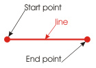
Line
Type: LINE (class name AcDbLine) Fig. 1.
 |
| Fig. 1 |
The object has two parameters: start point and end point. The position of the points in a drawing is defined by three coordinates: X,Y,Z. For two-dimensional drawings, the Z coordinate is usually neglected. Changing the position of the points on a plane relative to each other changes the length of the line.
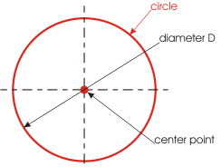
Circle
Type: CIRCLE. (class name AcDbCircle) Fig. 2.
 |
| Fig. 2 |
The geometry of the object is specified by two parameters: center point and diameter D. The position of the center point in a drawing is defined by three coordinates: X,Y,Z.
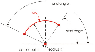
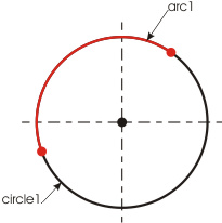
Arc
Type: ARC (class name AcDbArc) Fig. 3.
 |
| Fig. 3 |
The geometry of the object is specified by four parameters: center point, radius R, start angle, and end angle. The position of the center point in a drawing is defined by three coordinates: X,Y,Z. The angle value is specified in radians.
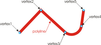
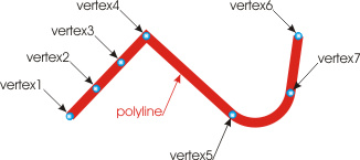
Polyline
Type: LWPOLYLINE (class name AcDbPolyline) Fig. 4.
 |
| Fig. 4 |
Polyline is a complex object, which consists of vertices linked by segments. The position of a polyline vertex in a drawing is defined by two coordinates: X,Y.
Unlike the above mentioned objects, polyline allows setting width to its segments (polyline width). Width can be specified by both variables (value varying from one vertex to another) and constants. In the vast majority of cases, polyline typically has a constant width throughout its length.
Polyline segments can be linear and arcuate, depending on the bulge factor, which defines the crown of the segment. When bulge = 0, the segment is linear.
As you can see it on the figure, there is an arcuate segment with bulge not equal to 0 between vertices 3 and 4. For all the other segments, bulge = 0.
Another typical feature of polyline is that it can form a closed loop. In this case, in terms of visual appearance, that means adding another segment linking the first and the last vertices.
| Definition of optimized drawing |
Any 2-D drawing created in AutoCAD environment basically consists of the above mentioned elementary objects, namely, lines, circles, and arcs. How efficiently user positions those objects in a drawing defines that user's professional excellence. A skilled user always seeks to minimize the number of objects involved in the drawing. Here we come to the definition of optimized drawing:
Terminology. Optimized drawing is a drawing that involves the smallest possible number of elementary objects (entities) for its graphical representation.
And cumulative use of means and methods, producing an optimized drawing, makes the essence of drawing optimization. |
Filleting different entities with each other woves the image of a drawing. There are various ways objects in a drawing can fillet with each: line with line, line with arc, arc with arc, etc. Let's review some of the simplest types of filleting two or more objects and the possibility of optimizing them.
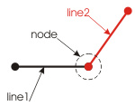
Filleting line with line
Figure 4a shows the filleting of two lines (line1 and line2) situated at an angle to each other.
 |
 |
| Fig. 4a |
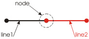
Fig. 4b |
Connecting to one another at some point, the objects form a node.
Figure 4b shows two lines that also fillet with one another and form a node, but these lines (unlike in the previous example) are collinear on one line.
If we analyze the two examples for possible optimization of these objects, it becomes clear that the two lines shown on Fig. 4a cannot be replaced with a single object (now we do not consider replacing with polyline LWPOLYLINE).
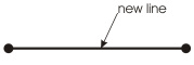
This is not the case for the lines shown on Fig. 4b. This combination of objects, as a result of optimization, can be replaced with a single object (line). Thus, we would have the following (see Fig. 5):
After the optimization, instead of two lines, line1 and line2, we have obtained a single new object, "new line".
Let's review filleting a greater number of lines with each other.
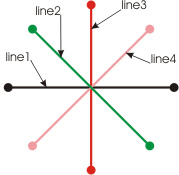
Figure 6 shows a figure formed of eight "line" objects.
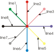 |
| Fig. 6 |
All those objects fillet in a single point, forming a node in the central part of the figure. Relative to the node, the lines are arranged evenly in a circle with angular increments of 45 degrees.
Let's analyze these objects for possible optimization.
Given the number of objects, uniformity of their arrangement in the circle and, as consequence, their pairwise codirection, it becomes clear that this set of objects could be represented otherwise and would require a much smaller number of same-type entities for its display. In other words, we would get the following (see Fig. 7):
 |
 |
| Fig. 7 |
Thus, to display the original drawing shown on Fig. 6, it is not really necessary to use 8 "line" objects; it is sufficient to use just four of them.
Now, let's review the cases when the lines, filleting with each other, do not form a node. In terms of optimization, interesting cases are those shown on Fig. 8a and Fig. 8b:
 |
 |
| Fig. 8a |
Fig. 8b |
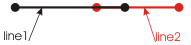
Figure 8a shows two collinear lines located on a single line, where line2 is smaller than line1 and is completely inside it (as a particular case of this example: both lines can completely match). It is clear that line2, in terms of optimization, is a redundant object, not carrying any information content. Hence, in the process of optimization, that object is to be removed; thus, we would get the following:
Figure 8b shows the case where two collinear lines, not forming a node, are positioned with some overlap on top of each other. It is clear that this set of objects can also be optimized by the replacement with a single entity (see Fig. 10):
Filleting arc with arc
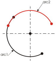
Similarly to lines, arcs can also form linked chains. Figure 11 shows an example of such complex arc consisting of two arcs, arc1 and arc2.
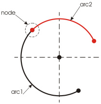 |
| Fig. 11 |
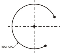
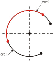
Optimization of filleted arcs requires meeting two conditions: matching center points and equal arc radiuses. Once these requirements are met, our complex object can be easily transformed into a single entity (new arc), see Fig.12.
|
 |
| Fig. 12 |
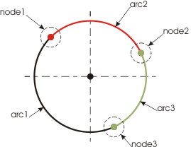
Let's review the case when arcs form a closed object; see Fig.13:
 |
| Fig. 13 |
The figure shows that the closed object consists of three arcs. All of them fillet with each other, forming three nodes – node1, node2, and node3, – have a common center point, and identical circle radiuses.
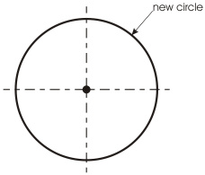
When a closed object consisting of several arcs is a circle, the optimization of that complex object comes down to the removal of all of its components and replacing those with a new CIRCLE entity. The result of the transformation is shown on Fig. 14:
|
 |
| Fig. 14 |
Just as in the case of lines (see Fig. 8 a, b) two or more arcs with identical radiuses and a common center point can fillet with each other without forming a node. Thus, the following 2 cases (see Fig. 15 a, b) allow optimization:
 |
 |
| Fig. 15a |
Fig. 15b |
Both these cases, as in the example shown on Fig. 12, can be transformed into a sigle ARC object.
Filleting circle with circle
Optimization of two circles can be implemented only when the following two conditions are met:
- Center point positions (coordinates) of both circles match.
- Radiuses (diameters) of both circles are equal.
In other words, when these parameters of two or more circles match, in a drawing we visually see only one CIRCLE object. That makes it completely clear that the optimization process in this case comes down to the identification and removal of redundant objects of this type.
Filleting circle with arc
Filleting a circle with an arc when optimization makes sense is shown on Fig. 16:
 |
| Fig. 16 |
Such filleting is a particular case of the above mentioned filleting two circles and, respectively, the conditions when the optimization is possible are similar to those described in that section; i.e., arc1 has the center point matching the center point of circle1, and the circle radius of the arc is equal to the radius of the circle. Thus, the optimization in this case comes down to the identification and removal of all arcs lying on the circle.
Optimizing polylines
The optimization of polylines ultimately comes down to the identification and removal of redundant vertices. Therefore, there are two possible cases of interest. In the first case, polyline has 3 or more vertices forming several codirectional segments (Fig. 17), and the optimization in this case is carried out within a single object.
 |
| Fig. 17 |
As the figure shows, vertices 1,2,3,4 are located on the same line and thus form 3 collinear segments. Clearly, two of the four vertices contain redundant information; therefore, in terms of optimization, the three segments are easily transformed into one by removing the two vertices in the middle (see Fig. 18).
|
|
| Fig. 18 |
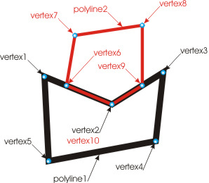
In the second case, in the process of optimization we identify fully or partially overlapping segments belonging to two or more polylines. Figure 19 shows a portion of a drawing displaying two closed polylines. Polyline 1 consists of vertices 1,2,3,4,5. Polyline 2 consists of vertices 6,7,8,9,10.
 |
| Fig. 19 |
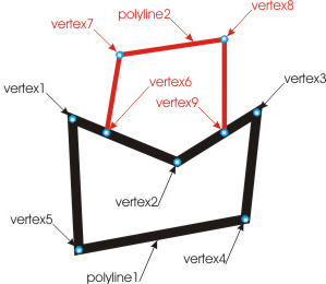
Both polylines osculate each other through two polygonal segments; besides, as the figure shows, there is an evident match of two vertices, 2 and 10. The osculating segments, 1-2 and 6-10, just as 2-3 and 9-10, overlap each other. The optimization of polylines in this case comes down to the identification of such overlaps and removal of the respective vertices located within the area of overlap. Therefore, in our case, after the optimization we obtain (see Fig. 20):
|
 |
| Fig. 20 |
As the figure shows, after the optimization polyline 2 loses its vertex 10 and the two segments, 6-10 and 9-10, and thus becomes open. Polyline 1 retains its original appearance.
|